
By Artur Loorpuu
A technical look at what a machine can reliably know from each of the three forms a P&ID usually takes, and what the published evidence says about closing the gap.
Reading time: ~14 min · Audience: process, instrumentation and digitalisation engineers
Abstract
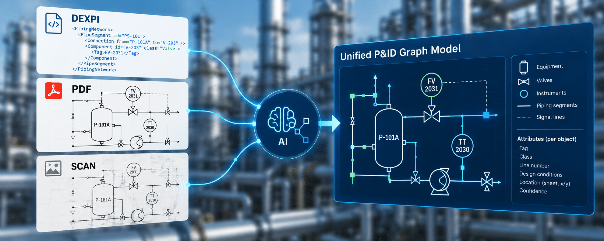
To software, a piping and instrumentation diagram (P&ID) is a graph. Equipment, nozzles, valves and instruments are the nodes. Pipe segments and signal lines are the edges. Tags, line classes and design conditions are the attributes. Any useful automated reasoning over a P&ID has to recover that graph first, whether it’s tracing an isolation boundary, listing what sits downstream of a failed pump, or preparing HAZOP nodes. Plants hold their P&IDs in three very different forms. Some are smart exports in the DEXPI standard, which carry the graph explicitly. Some are vector PDFs, which carry exact geometry and text, with the meaning left implicit. Many are raster scans, which carry only pixels. This post compares what each form encodes, reviews the recent published results on recovering the graph from scans, and argues for one design principle: whatever the source, converge on a single explicit graph model, and keep a confidence value on every edge.
1. The P&ID is a graph. The file usually isn’t.
An engineer reading a P&ID resolves a great deal without noticing. A line that crosses another without a dot is not a junction. A dashed line is a signal, not a pipe. An off-page connector means the line continues on sheet 14. The tag bubble next to a valve belongs to that valve and not to the pipe beside it. All of this is interpretation, and it’s the interpretation, not the drawing, that answers questions like “what do I have to close to isolate P-101A?”
We can define the target precisely. A usable P&ID model needs at least:
| Element | Minimum content |
| Nodes | Equipment, nozzles, piping components (valves, reducers, spectacle blinds), instruments, off-page connectors |
| Edges | Piping segments (nozzle-to-component, component-to-component) and signal/information flows |
| Identity | A stable ID per object, plus the plant tag (e.g. P-101A, FV-2031) |
| Direction | Flow direction on piping, source → sink on signal lines |
| Attributes | Line number, nominal diameter, piping class, design pressure/temperature, fail position, etc. |
| Provenance | Which sheet, which revision, and where on that sheet each object came from |
The three formats differ in which of these rows are explicit and which must be inferred. That is the whole story.
| DEXPI (Proteus / DEXPI XML) | Vector PDF | Raster scan | |
| Object identity | Explicit | Inferred (geometry clusters) | Inferred (detection) |
| Object class | Explicit, linked to a reference data library | Inferred (symbol matching) | Inferred (symbol classification) |
| Text / tags | Explicit, bound to objects | Exact strings, but unbound | OCR, noisy and unbound |
| Topology (edges) | Explicit | Inferred from line endpoints | Inferred from pixels |
| Flow direction | Explicit | Inferred (arrows) | Inferred (arrows) |
| Non-graphical attributes | Explicit where the source tool held them | Only if printed on the sheet | Only if printed and legible |
| Main error source | Source-tool data quality | Geometric ambiguity | Everything above, plus image noise |
2. DEXPI: the graph, written down
What it is. DEXPI (Data Exchange in the Process Industry) is a vendor-neutral information model for P&IDs. It was launched in 2011 by a group of owner-operators (BASF, Bayer, Evonik), CAE vendors (Autodesk, AVEVA, Bentley, Intergraph, Siemens), research partners (AIXCape, RWTH Aachen) and an engineering contractor (Air Liquide) [1]. The model has its roots in ISO 15926, and object classes can be linked to a reference data library.
Where the standard stands in 2026. The DEXPI P&ID Specification 1.4 was released at the end of 2024. DEXPI Process 1.0, which covers BFDs and PFDs, followed at the end of 2023. On 10 October 2025 the association published DEXPI 2.0, which packages the plant (P&ID) and process (PFD/BFD) models together for the first time. It introduces “DEXPI XML”, a simplified UML-based serialisation that replaces the earlier Proteus schema. The plant model content is unchanged from 1.4, so existing P&ID integrations are not invalidated [2][3]. The specification is published openly on GitLab under CC BY 4.0 [2]. DEXPI also has an OPC UA companion specification [4] and an Asset Administration Shell submodel (IDTA 02012-1-0) [5]. Those two matter if you want P&ID structure to sit next to live data and asset records instead of in a separate silo.
What it encodes. In a DEXPI file, a piping network is a set of segments. Each segment’s Connection element references the IDs of the objects at its ends, such as a nozzle on a vessel or a pipe tee, and the piping components inside the segment are listed in sequence. Every object carries a class (ComponentClass) and a URI into a reference data library such as the POSC Caesar RDL (ComponentClassURI). Engineering attributes like tag names and line numbers are serialised as GenericAttribute elements [17]. Instruments and control loops are first-class objects, and so are the signal lines between them. Graphical information (position, symbol, label placement) sits alongside the semantic content, not in place of it. The following is a simplified excerpt in Proteus XML, with RDL URIs and graphics omitted:
<Equipment ID=”pump1″ ComponentClass=”CentrifugalPump” ComponentClassURI=”…”>
<GenericAttributes Set=”DexpiAttributes”>
<GenericAttribute Name=”TagNameAssignmentClass” Value=”P-101A” Format=”string”/>
</GenericAttributes>
<Nozzle ID=”nozzle1″ ComponentClass=”Nozzle” ComponentClassURI=”…”/> <!– discharge –>
</Equipment>
<PipingNetworkSystem ID=”pns1″ ComponentClass=”PipingNetworkSystem”>
<GenericAttributes Set=”DexpiAttributes”>
<GenericAttribute Name=”LineNumberAssignmentClass” Value=”P-1021″ Format=”string”/>
</GenericAttributes>
<PipingNetworkSegment ID=”seg1″ ComponentClass=”PipingNetworkSegment”>
<PipingComponent ID=”valve1″ ComponentClass=”GateValve” ComponentClassURI=”…”/>
<Connection FromID=”nozzle1″ ToID=”nozzle2″/> <!– pump discharge → vessel inlet –>
</PipingNetworkSegment>
</PipingNetworkSystem>
Recovering the graph from this is a parse rather than a recognition problem, and it’s deterministic. Open tooling exists: pyDEXPI, from the Process Intelligence group at TU Delft, provides a Pydantic implementation of the data model. It includes a loader for Proteus XML, a converter to a NetworkX graph, and a generator for synthetic DEXPI P&IDs [6][7].
What DEXPI doesn’t guarantee. Three caveats, all from experience rather than from the specification:
- Garbage in, structured garbage out. A DEXPI export is only as smart as the source project. If a designer drew a line in a smart P&ID tool without connecting it to the nozzle, which is common under schedule pressure, the export faithfully reports a disconnected segment. The format makes the error visible, which is valuable, but it doesn’t fix it.
- Implementation coverage varies. The DEXPI software register lists tools that do import and export (e.g. AVEVA PID, COMOS P&ID, Engineering Base, CADMATIC, X-Visual). It also lists export-only tools, such as AVEVA Diagrams, AutoCAD P&ID and older Smart P&ID versions, and tools pinned to specific versions (e.g. CADMATIC on 1.3) [8]. “Supports DEXPI” is therefore a claim to test with a round-trip on your drawings, not a checkbox.
- Brownfield reality. Many operating plants, especially older ones, don’t have their P&IDs in a smart tool at all. For them, DEXPI is a target format, not a source format. The rest of this post is about that gap.
3. Vector PDF: exact geometry, implicit meaning
A PDF exported from CAD is often treated as “just a picture”. It isn’t. For brownfield plants it may be the most information-rich source available. Its content stream holds exact vector paths (line segments, arcs, Bézier curves), and usually real text objects with their glyph positions and font information. For digitisation that’s a large advantage over a scan:
- Text is exact. If the text wasn’t converted to outlines on export, tag strings can be read directly with no OCR error at all. That fixes the weakest link in scan pipelines (see §4).
- Geometry is exact. There’s no noise, skew, bleed-through or broken strokes. Endpoints are floating-point coordinates, so “does this line touch that nozzle?” becomes a tolerance question, not a pixel-segmentation question.
What the PDF doesn’t carry is the semantic layer: which strokes form one valve, which label belongs to which object, which lines actually connect. That layer has to be reconstructed, and a recognition pipeline has to solve the following:
| Challenge | Why it arises |
| Symbols are exploded | A valve block becomes a loose set of strokes. Symbols have to be re-identified by geometric pattern matching or by a detector running on a rendered image. |
| Lines are fragmented | One pipe run may be dozens of path segments, split at every text gap, dimension or layer change. Dashed signal lines arrive as hundreds of dashes. |
| Crossing vs junction | Two collinear-perpendicular segments that meet can be a tee or a crossing, and the difference is a drawing convention (a dot, a gap, a hop). The geometry alone doesn’t settle it. |
| Text is unbound | The string FV-2031 is exact, but which object it labels is still a proximity guess. |
| Text outlined | Some export settings turn text into curves, which silently removes the exact-text advantage. |
| Off-page continuity | Connectors are just text and a symbol. Joining sheets needs the connector labels to be resolved, which the PDF doesn’t do. |
Put plainly, a vector PDF moves the problem from perception to interpretation. That’s a large gain. The line-noise and OCR errors that dominate scan pipelines (§4) largely disappear, and what’s left is a well-posed reasoning problem over exact inputs. Published work on P&ID-specific vector parsing is much thinner than on scans. Most of the literature treats PDFs as images to be rendered [9]. We think this is the most under-exploited route to a machine-readable brownfield plant: in many document management systems, a large share of the “scanned” P&IDs turn out to be vector PDFs once someone checks.
3.1 What we are building
This is the route UReason is actively developing. Our recognition pipeline reads a PDF P&ID two ways. Where the file has vector content, it uses the drawing’s own geometry and text. Where it’s only a rendered image, which is typical of legacy PDFs, it works from the image. In both cases a locally hosted language model does the interpretation: grouping strokes into components, binding tags and line numbers to the objects they describe, and reconstructing how everything connects. Because of this, the same pipeline covers both the clean CAD exports and the image-only PDFs that make up much of a brownfield archive. The model runs inside the customer’s environment, so the drawings never leave their network. For plants whose governance rules out sending P&IDs to a cloud API, that’s a precondition, not a feature.
Figure 1 shows the pipeline’s output on the official DEXPI example P&ID, the public example drawing published by the DEXPI association. Components, tags, line labels and design parameters are identified automatically, and the connecting segments are reconstructed. Because a machine-readable DEXPI version of this drawing exists, it’s also a natural reference for checking recognition output against ground truth. How the pipeline works, and how we measure it, deserves its own post. That one is coming.
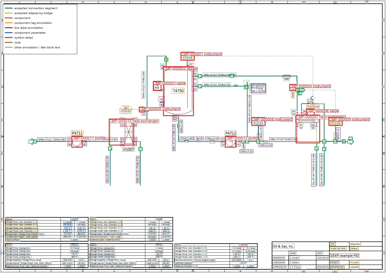
Source: “C01 DEXPI Reference P&ID” (C01V04-VER.EX01), © DEXPI e.V., from the DEXPI Public Example PIDs repository [18], licensed under CC BY 4.0. Changes: recognition overlay and legend added by UReason.
4. Raster scans: what the literature actually reports
Scans are the hardest case and the most researched. Four results give a fair picture of the state of the art, and the conditions behind each number matter as much as the number itself.
4.1 High scores on in-distribution data. Kim et al. (2022) built an end-to-end pipeline trained on a large labelled corpus of 75,031 symbol, 10,073 text and 90,054 line instances. They report [10]:
| Task | Precision | Recall |
| Symbols | 96.65 % | 96.40 % |
| Text | 90.65 % | 92.16 % |
| Lines | 95.25 % | 87.91 % |
| Topology reconstruction | 99.56 % | 96.07 % |
These are strong numbers. They come from a test set of five P&IDs drawn in the same conventions as the training data. The authors also state that attribute values of plant items cannot be reliably extracted from the image, and have to come from manual input or other sources [10]. Text sits about 5 points below symbols. Line recall (87.91 %) sits about 8 points below line precision. Missed lines are missed edges.
4.2 The drop on public real-world data. Stürmer et al. (IEEE DSAA 2025) released PID2Graph, the first public P&ID benchmark with graph-level ground truth. It combines synthetic diagrams with 12 manually annotated real P&IDs from the OPEN100 reactor design [11][12]. Their transformer-based model (Relationformer) extracts symbols and connections jointly:
| Node AP | Edge mAP | |
| Relationformer, synthetic | 96.89 % | 88.95 % |
| Relationformer, real (OPEN100) | 83.63 % | 75.46 % |
| Modular baseline, synthetic | 85.16 % | 50.26 % |
| Modular baseline, real (OPEN100) | 52.14 % | 45.89 % |
Two lessons follow. First, learning nodes and edges jointly beats the classic detect-symbols-then-trace-lines pipeline by about 30 points on real edges. Second, even the better model loses about 13 points of node AP and 13 points of edge mAP going from synthetic to real drawings. The authors name the causes: symbols cut at patch boundaries, a confusable “general” symbol class, large symbols, and annotation uncertainty. They also note that OPEN100 has no dashed lines [12]. Real plants have plenty.
4.3 Synthetic data helps, up to a point. Prasad and Mahapatra (2026) generated 665 synthetic P&IDs whose pipe topology is seeded from real drawings, and trained without any real images. They reached 63.8 ± 3.1 % edge mAP on OPEN100, roughly 8 points below a model trained on real data. Earlier template-based synthetic data scored about 33 %. Gains plateaued after about 400 synthetic images, and the authors identify seed diversity as the binding constraint [13].
4.4 The evaluation base is thin. The Digitize-PID pipeline (Paliwal et al., PAKDD 2021) was validated on 500 synthetic diagrams and 12 real, private sheets [14]. The main public real-world benchmark is 12 sheets. For a field that wants to claim “industrial readiness”, that’s a small evidence base, and practitioners should read any headline accuracy figure with the test set in mind.
Why edge accuracy dominates. Object-level precision and recall understate how errors reach the questions people actually ask. A path query, “is there a flow path from T-201 to the flare header?”, is only correct if every edge along the path is correct. As an illustrative calculation, assume each edge is independently correct with probability p and the path has k = 10 edges:
| p (per-edge correctness) | P(10-edge path fully correct) = p¹⁰ |
| 0.99 | 0.90 |
| 0.95 | 0.60 |
| 0.75 | 0.06 |
The independence assumption is a simplification, and edge mAP isn’t literally a per-edge probability. The shape of the curve is the point: errors compound multiplicatively along paths. The two error types also have different costs. A missed junction splits a network and produces false “no path” answers. A false junction, such as a crossing read as a tee, invents a flow path. For isolation planning that’s the more dangerous error, because it can make an isolation look complete when it isn’t.
5. Why the graph matters for LLMs too
The same logic applies when a language model sits on top. Alimin and Schweidtmann (2026) compared LLM question-answering on one DEXPI example P&ID. The model saw the P&ID three ways: as an image, as the raw Proteus XML, and as a knowledge graph built with pyDEXPI and queried through graph retrieval. On 19 question-answer pairs, GPT-5 scored [15]:
| Input representation | Avg. accuracy | Cost per task |
| Raw image | 0.76 | — |
| Raw Proteus XML | 0.89 | $0.175 |
| Knowledge graph (ContextRAG) | 0.94 | $0.027 |
The authors summarise this as an 18 % accuracy gain over images and an 85 % token/cost reduction against ingesting the smart P&ID file directly. They also report that small open-weight models “still struggle to interpret knowledge graph formats”, and needed additional vector/path retrieval to recover accuracy [15]. The sample is small: one diagram and 19 questions. The direction matches everything above. Explicit structure beats pixels, and a curated graph beats a raw dump even of good structure. A second line of work uses multimodal LLMs directly on drawings, in two stages that separate visual extraction from topology reconstruction [16]. That’s promising, but it hasn’t yet been reported against a graph-level benchmark like PID2Graph.
6. A design principle: converge on one graph, and carry the uncertainty
Taken together, the evidence points to a pipeline shape that doesn’t depend on which of the three formats a site happens to have:
- One target model. DEXPI files, vector PDFs and scans should all land in the same explicit graph schema. The DEXPI plant model is the obvious candidate, since it’s open, maintained and already emitted by the major CAE tools. Downstream reasoning (path tracing, isolation, HAZOP node preparation, LLM question-answering) then never needs to know where a node came from.
- Confidence per element. An edge parsed from DEXPI has confidence ≈ 1, subject to source quality. An edge inferred from a scan might be 0.8. Keep that number on the edge. Propagate it into answers (“this path depends on two low-confidence connections on sheet 7”), rather than rounding every edge to true or false.
- Engineering rules as a validator. Domain rules catch whole classes of recognition error for free. A pump has one suction and one discharge. A control valve has a signal input. Line numbers are continuous along a run. Off-page connectors come in pairs. Flow direction is consistent across a segment. Digitize-PID already uses domain-knowledge validation in this way [14].
- Review where it’s uncertain. Human checking time is the scarce resource. Rank review by consequence × uncertainty, for example low-confidence junctions on lines that bound an isolation. Don’t spread it evenly across a sheet.
- Provenance on everything. Every node and edge keeps a link back to the sheet, the revision and the pixel or vector region it came from. That lets an engineer check an answer in seconds, and it’s how trust in the system is earned.
In summary: DEXPI solves the representation problem but not the brownfield problem. Scans are improving fast but are measured on very small benchmarks. Vector PDFs sit in between, and are the most promising route to bringing existing plants into the same graph model. The practical path is to treat format as a property of the evidence, not of the model.
How this connects to Process Insights and Asset Insights
UReason’s Process Insights is built on the argument of this post. It turns P&IDs into a system engineers can query in plain language, together with FMEA/FMECA sheets, SOPs, manuals and live process data. It “reasons across equipment, valves, instruments, and flow paths – the way an experienced engineer would – not just as isolated documents.” Tracing upstream and downstream impact, preparing HAZOP and risk scenarios, and troubleshooting a deviation are all path questions over the plant’s topology. Answers link back to the original sources, so an engineer can check them. That’s why the quality of the underlying P&ID model, and the recognition work described in §3.1, matter so much to us.
Asset Insights applies the same idea to the individual asset. It turns manuals, procedures, specifications and spare-parts information into structured, searchable knowledge, including Asset Administration Shell (AAS) models and Digital Product Passports. Together, the two link the process view (how things connect) with the asset view (what each thing is and how to maintain it). That’s the same bridge that standards like the DEXPI AAS submodel [5] are designed to formalise.
Further reading on the UReason blog:
- The P&ID Has the Answer. Getting It Out Is the Problem.
- From Static Diagrams to Living Systems: Making P&IDs Queryable with LLMs
- The Bowtie You Never Had Time to Build
Turn Your P&IDs Into Actionable Process Insights
Book a call with Artur Loorpuu, Senior Solutions Engineer at UReason, to explore how UReason can turn your existing P&IDs and engineering data into structured, queryable insights for tracing flow paths, understanding process relationships, and supporting engineering decisions.

References
- OPC Foundation, “DEXPI”, markets & collaboration page. https://opcfoundation.org/markets-collaboration/dexpi/
- DEXPI e.V., “DEXPI 2.0 Specification Published — A New Standard for Process Industry Data Exchange”, 2025. https://dexpi.org/dexpi-2-0-specification-published-a-new-standard-for-process-industry-data-exchange/
- Tolksdorf, G., Cameron, D. B., Theißen, M., “DEXPI 2.0: Synergistic Integration of PFD and P&ID in a Unified Digital Model”, Chemie Ingenieur Technik 97(11–12), 1065–1069, 2025. https://doi.org/10.1002/cite.70009
- OPC Foundation, “OPC Unified Architecture for DEXPI” (OPC 30250). https://reference.opcfoundation.org/specs/OPC-30250/5.1
- IDTA, “IDTA 02012-1-0 Information Model for P&I Diagrams based on DEXPI Standard”, 2023. https://industrialdigitaltwin.org/wp-content/uploads/2023/09/IDTA-02012-1-0_Submodel_DEXPI.pdf
- Goldstein, D. P., Schulze Balhorn, L., Alimin, A. A., Schweidtmann, A. M., “pyDEXPI: A Python framework for piping and instrumentation diagrams (P&IDs) using the DEXPI information model”, Systems and Control Transactions 4 (Proc. ESCAPE 35), 1365–1370, 2025. https://doi.org/10.69997/sct.139043
- Process Intelligence Research, pyDEXPI (GitHub, AGPL-3.0). https://github.com/process-intelligence-research/pyDEXPI
- DEXPI e.V., “Software” register. https://dexpi.org/software/
- Moreno-García, C. F., Elyan, E., Jayne, C., “New trends on digitisation of complex engineering drawings”, Neural Computing and Applications 31(6), 1695–1712, 2019. https://doi.org/10.1007/s00521-018-3583-1
- Kim, B. C., Kim, H., Moon, Y., Lee, G., Mun, D., “End-to-end digitization of image format piping and instrumentation diagrams at an industrially applicable level”, Journal of Computational Design and Engineering 9(4), 1298–1326, 2022. https://doi.org/10.1093/jcde/qwac056
- PID2Graph dataset, Zenodo. https://zenodo.org/records/14803338
- Stürmer, J. M., Graumann, M., Koch, T., “From Engineering Diagrams to Graphs: Digitizing P&IDs with Transformers”, IEEE DSAA 2025. https://arxiv.org/abs/2411.13929
- Prasad, S., Mahapatra, P., “SynthPID: P&ID digitization from Topology-Preserving Synthetic Data”, 2026. https://arxiv.org/abs/2604.16513
- Paliwal, S., Jain, A., Sharma, M., Vig, L., “Digitize-PID: Automatic Digitization of Piping and Instrumentation Diagrams”, PAKDD 2021. https://arxiv.org/abs/2109.03794
- Alimin, A. A., Schweidtmann, A. M., “GraphRAG for Engineering Diagrams: ChatP&ID Enables LLM Interaction with P&IDs”, 2026. https://arxiv.org/abs/2603.22528
- Zhu, B., Duong, S., Vyas, J., Mercangöz, M., “From P&ID Drawings to Process Graphs: A Multimodal Language Model Approach”, 2026. https://arxiv.org/abs/2607.19568
- DEXPI e.V., “Implementation in Proteus Schema”, DEXPI P&ID Specification 1.4. https://dexpi.org/static/pid_specification_1.4/concepts/proteus.html
- DEXPI e.V., “Public Example PIDs”: C01 DEXPI Reference P&ID (C01V04-VER.EX01), CC BY 4.0. https://gitlab.com/dexpi/TrainingTestCases