Smoothening your Predictions with Splines

Data-based prediction with a Smoothing Splines model

This article deals with a frequently occurring problem with pumps – sudden drops in the flow rate. This can have many reasons, ranging from technical problems inside the respective pump to problems in the process. It is important to take all these indicators into account when trying to predict the sudden drops in flow rate. This article showcases a step-by-step overview of the approach to such a problem, as well as an interesting algorithm that captures the flow rate pattern surprisingly well!

It is worth noting why predicting sudden drops and rises in flow rate is important. Although there is a multitude of possibilities, this article will highlight one of the most unwanted causes of flow drops: clogging. If the drops in flow rate are not recognized timely, the response might already be too late. This means in the worst-case scenario, that the pump is clogged. This might result in pump breakdown or at least lose a large part of its durability. The main goal is to have a model that predicts this timely.

As for every data-based prediction task, the first step is exploring the data and deciding what features will be used. Then, the data is preprocessed to be suitable as input for the chosen model. The prediction model will be a smoothing splines model, which is used to predict numerical data that has a rather noisy distribution. The article further elaborates on this model.

Data Exploration

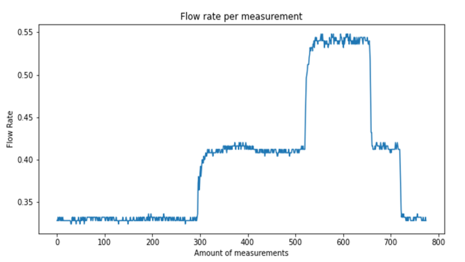
We use a dataset from the Flow Center of Excellence, an experimental flow loop where the pump is located. The dataset consists of 120 features in total. The dataset contains a lot of features that will not be used for this case, such as warning codes or categorical state variables. For this model, we solely focus on raw numerical data, as smoothing splines are a regression-based model, which uses numerical data as input to predict a numerical value (in this case, the flow rate). The figure below shows the behaviour of the flow rate data over time.

Model setup

As mentioned earlier, smoothing splines will be used as the model to predict the behaviour of the flow rate. Below is a stepwise approach to creating the prediction model, starting with normalizing the data between 0 and 1 to have equal weights for all features. The next step is to divide the dataset into a training and test set. The training set will be used to fit the model and the test set is used to see how well the trained model performed on its prediction task.

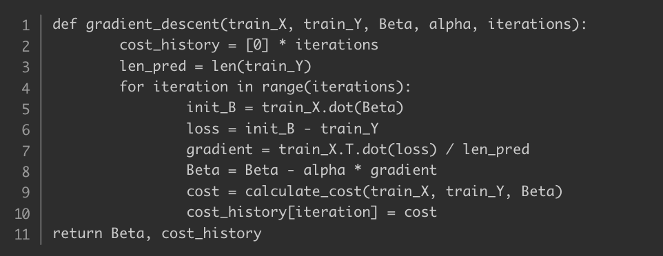
Next, a cost function has to be defined, which will be minimized as the objective for the optimization task. For more clarification, the Mean Squared Error (MSE) is used for the cost function, as gradient descent is for optimization function. Below is the Python code for the gradient descent function.

Additionally, smoothing splines need to be added to the model to remove the noise in the prediction. For this example, natural cubic splines are chosen. This article does not go into full mathematical detail of this algorithm but gives an overview of the working of splines. The idea is as follows: the least-squares algorithm produced a fitted function.

This function is then divided into sub-functions, referred to as knots. These knots will then all be individual function representations, with the only constraint that its consecutive knot has the same second derivative.

This means that the slope of the knot is equal to the slope of the next knot at its transition point. The following figure represents a different amount of knots to show a visual explanation of the above mentioned.

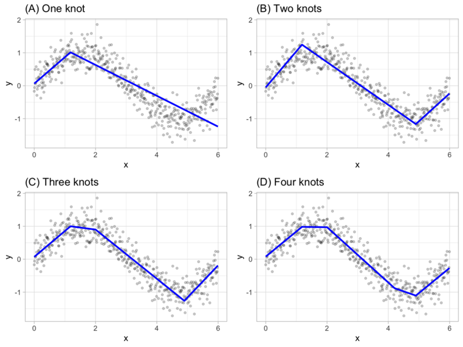
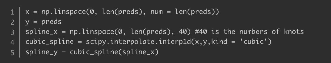
The goal here is to have a group of knots that all represent their own ‘region’ within the prediction, which are then connected to represent a smooth curve. The Python code below shows the setup of the cubic spline interpolation.

Finally, it remains to observe whether the model did a good job at predicting the flow rate of the pump. To this end, the algorithm is implemented in APM Studio. UReason’s APM Studio provides a variety of AI techniques and tools that help you quickly set up and train your own APM solutions. These solutions allow you to provide Condition Based Monitoring, Predictive Failure Models, Probabilistic Risk Models and more for your assets. Within APM Studio, a processing rule is created, where a REST call is sent to a server where the algorithm is accessible. This way, any algorithm that is written can be accessed easily by using a REST node. The processing rule is shown below.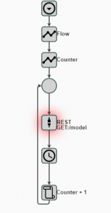

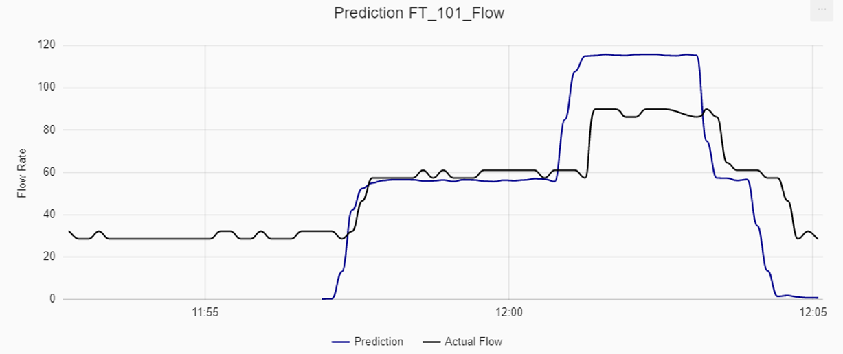
Previously, the article stated two main patterns that the model should capture. The first one was that the model should predict when the flow rate jumps to a new plateau. The second one was that the model should not react to small volatility. As can be observed in the figure below, this model did a great job in doing so. Of course, it can also be seen that the prediction is very reactive to these large drops, but this is not a problem as the main aim is to measure that the flow rate is in a new state.